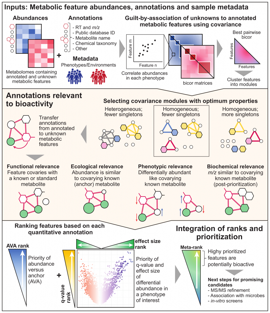
MACARRoN (Metabolome Analysis and Combined Annotation Ranks to pRioritize Novel bioactives) is a computational workflow for the systematic analysis of microbial community associated metabolomes towards prioritization of novel, potentially bioactive metabolites. Here, bioactivity indicates the likelihood of causal or consequential involvement in a phenotype or environment of interest. MACARRoN is based on the principle of guilt-by-association and uses correlated abundances (covariance) between metabolic features to transfer biologically meaningful annotations from annotated metabolites to unknown metabolic features in large-scale, untargeted metabolomes. For each metabolic feature, MACARRoN evaluates quantitative indicators of bioactivity such as abundance versus covarying, abundant known metabolite aka anchor (AVA), and q-value and effect size of differential abundance in a phenotype of interest. Finally, it prioritizes metabolic features with respect to their bioactivity based on the meta-rank of the aforementioned indicators of bioactivity. MACARRoN is available as a Bioconductor package and can be run via both command line and R.
User manual || Tutorial || Forum
Citation:
Amrisha Bhosle, Sena Bae, Yancong Zhang, Eunyoung Chun, Julian Avila-Pacheco, Ludwig Geistlinger, Jonathan Glickman, Monica Michaud, Levi Waldron, Clary Clish, Ramnik J. Xavier, Hera Vlamakis, Eric A. Franzosa, Wendy S. Garrett*, Curtis Huttenhower*. "Identifying Novel Bioactive Metabolites in Inflammatory Bowel Disease" [in preparation]
Feel free to link MACARRoN in your Methods: http://199.94.60.28/macarron/
Please direct your questions to the biobakery discussion Forum.
Overview

Getting Started
Requirements
- R software
- R CRAN packages: WGCNA, dynamicTreeCut, ff, plyr, stats, psych, data.table, xml2, RCurl, RJSONIO, logging, optparse
- R Bioconductor packages: SummarizedExperiment, BiocParallel, DelayedArray, Maaslin2
Installing MACARRoN
Once you have the correct version of R, you can install MACARRoN with Bioconductor.
if(!requireNamespace("BiocManager", quietly = TRUE))
    install.packages("BiocManager")
BiocManager::install("Macarron")
You may encounter an error message that states:
Warning message:
package ‘Macarron’ is not available (for R version x.x.x)
This can be due to one of two reasons:
- Your R version is too old. Check this with
sessionInfo()- if it is older than 3.6, download the most updated version per instructions above. - You have an older version of Bioconductor. MACARRoN requires Bioconductor >= 3.10. You can check your Bioconductor version with
BiocManager::version(). If the returned version is anything older than 3.10, you can update with:BiocManager::install(version = "3.10")
and then:BiocManager::install("Macarron")
Prioritization of bioactive metabolites with MACARRoN
MACARRoN Inputs
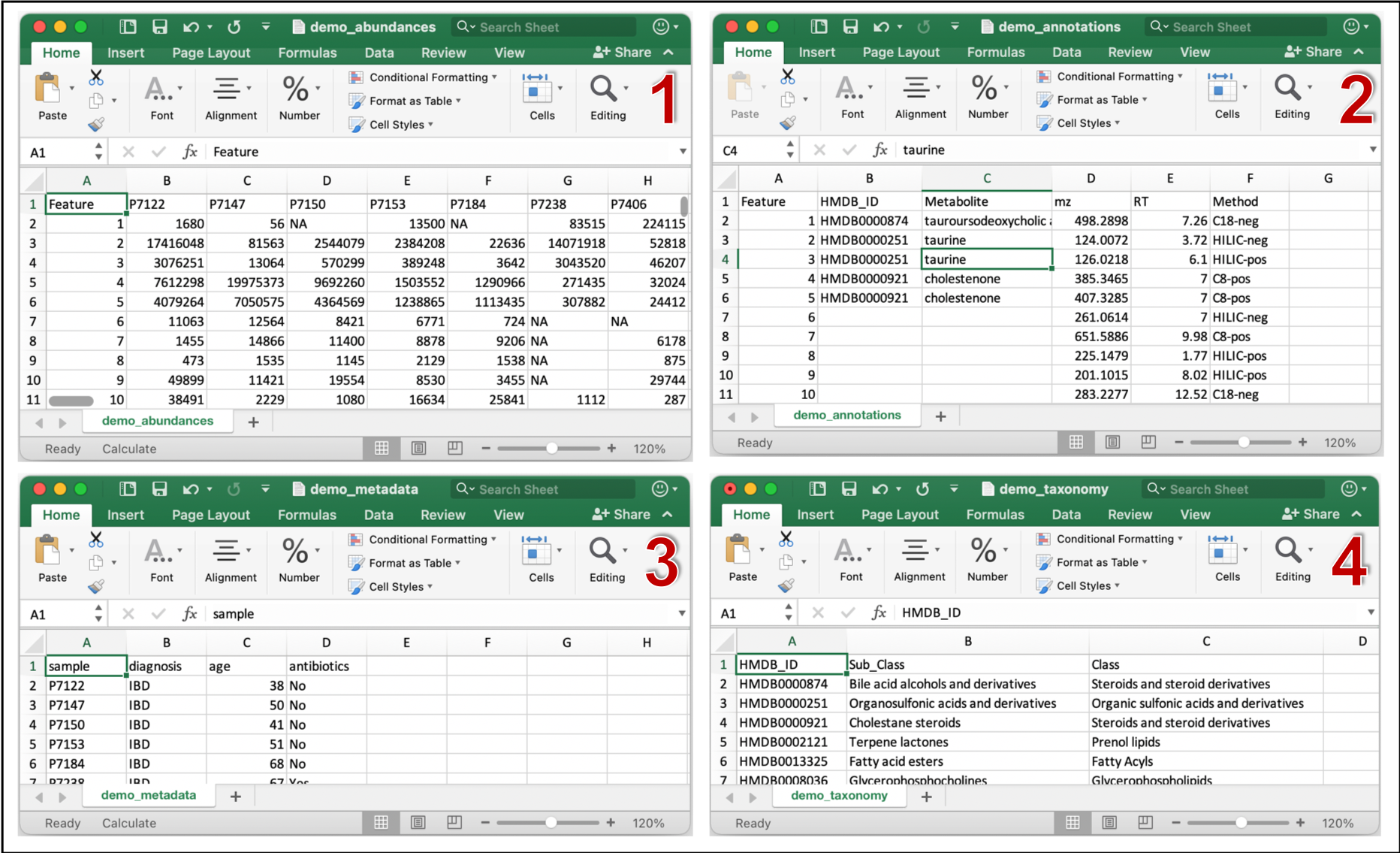
MACARRoN requires 4 comma-separated, appropriately formatted input files. The files and their formatting constraints are described below.
- Metabolic features abundance table
- Must contain features in rows and samples in columns.
- First column must identify features
- Metabolic features annotation table
- Must contain features in rows and annotations in columns.
- First column must identify features.
- Second column must contain either HMDB ID or PubChem Compound Identifier (CID) e.g. HMDB0304632 or 24749 for glucose. These will be available only for a small fraction of features in untargeted metabolomes resulting in several empty cells.
- Third column must contain the name of the metabolite.
- Fourth column must contain a continuous chemical property such as m/z or RT or shift/ppm.
- Other compound metadata can be listed column 5 onwards.
- Sample metadata table
- Must contain samples in rows and metadata in columns.
- First column must identify samples.
- Second column must contain categorical metadata relevant to prioritization such as phenotypes, exposures or environments.
- Chemical taxonomy table
- First column must contain the HMDB ID or PubChem CID. IDs must be consistent between annotation and taxonomy tables.
- Second and third columns must contain chemical subclass and class of the respective metabolite.
- If you do not have this file, please see instructions under Advanced Topics on how to generate this file using the annotation table and MACARRoN utility
decorate_ID.
Example (demo) input files can be found under inst/extdata folder of the MACARRoN source. These files were generated from the PRISM study of stool metabolomes of individuals with inflammatory bowel disease (IBD) and healthy "Control" individuals. Control and IBD are the two phenotypes in this example. MACARRoN will be applied to prioritize metabolic features with respect to their bioactivity in IBD. The four input files are demo_abundances.csv, demo_annotations.csv, demo_metadata.csv, and demo_taxonomy.csv. Snapshots of each file are shown below.

Running MACARRoN in RStudio or R
Launch RStudio and in the R script window, enter:
rm(list=ls())
getwd()
setwd("~/Desktop")
dir.create("Macarron_demo") # Create a new directory
setwd("Macarron_demo") # Change the current working directory
getwd() # Check if directory has been successfully changed

#Load MACARRoN package into the R environment
library(Macarron)
?Macarron
Using CSV files as inputs:
prism_abundances = system.file("extdata", "demo_abundances.csv", package="Macarron")
prism_annotations = system.file("extdata", "demo_annotations.csv", package="Macarron")
prism_metadata = system.file("extdata", "demo_metadata.csv", package="Macarron")
met_taxonomy = system.file("extdata", "demo_taxonomy.csv", package="Macarron")
We can now apply MACARRoN to identify features that are potentially bioactive in IBD:
prioritized_output = MACARRoN(
    input_abundances = prism_abundances,
    input_annotations = prism_annotations,
    input_metadata = prism_metadata,
    input_taxonomy = met_taxonomy)
OR
Using dataframes as inputs:
abundances_df = read.csv(file = prism_abundances, row.names = 1) # setting features as rownames
annotations_df = read.csv(file = prism_annotations, row.names = 1) # setting features as rownames
metadata_df = read.csv(file = prism_metadata)
taxonomy_df = read.csv(file = met_taxonomy)

# Run MACARRoN
prioritized_output = MACARRoN(
    input_abundances = abundances_df,
    input_annotations = annotations_df,
    input_metadata = metadata_df,
    input_taxonomy = taxonomy_df)
MACARRoN output
By default, all files will be stored in a folder named MACARRoN_output inside the directory (Macarron_demo) that we initially created. The name of the output folder can be changed with the output argument. There are several output files/folders in MACARRoN_output, however the main prioritization results are stored in prioritized_metabolites_all.csv. Another file, prioritized_metabolites_characterizable.csv is a subset of prioritized_metabolites_all.csv and only contains metabolic features that covary with at least one annotated metabolite.
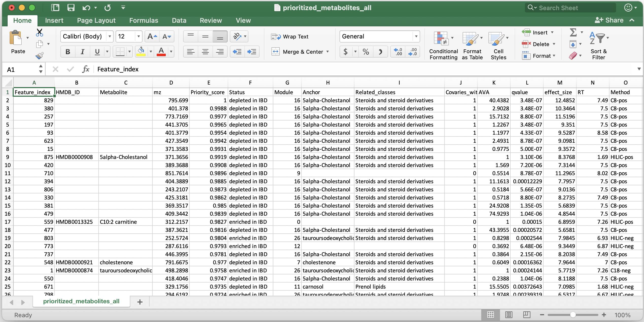
Shown below is a snapshot of prioritized_metabolites_all.csv: 25 metabolic features listed in the order of their priority in IBD.

The columns are :
- Feature_index: lists the identifier of the metabolic feature found in column 1 of abundance and annotation tables. In this example, it was serial numbers.
- HMDB_ID and Metabolite: Public database identifier and metabolite name from columns 2 and 3 of the annotation table.
- mz: The continuous numerical chemical property from column 4 of the annotation table.
- Priority_score: Priority score where 1 indicates most prioritized. Rank percentile is derived from the meta-rank of AVA, q-value and effect size.
- Status: Direction of perturbation (differential abundance) in IBD (phenotype of interest) compared to Control (reference phenotype).
- Module: ID of the covariance module a metabolic feature is a member of. Module = 0 indicates a singleton i.e., a metabolic feature that is not assigned to any module.
- Anchor: Metabolic feature that has the highest abundance in any phenotype (IBD or Control) e.g. 5alpha-Cholestanol had the highest abundance among all metabolic features in module 16. In modules containing both annotated (standard) and unannotated features, anchor is the most abundant annotated feature. If a metabolic feature is the only annotated one in its module, it automatically becomes the anchor. In modules containing all unannotated features, the one with the highest abundance is chosen as the anchor. This column helps in functional characterization or hypothesis generation.
- Related_classes: Chemical taxonomy of the annotated features that covary with a metabolic feature e.g. feature 829 covaries with metabolites that are steroids or their derivatives. This column also helps in functional characterization or hypothesis generation.
- Covaries_with_standard: 1 (yes) and 0 (no). Column specifies if the metabolic feature covaries with at least one annotated (standard) metabolite.
- AVA: Abundance versus anchor which is a ratio of the highest abundance (in any phenotype) of a metabolic feature and highest abundance of the covarying anchor. Naturally, the AVA of an anchor is 1.
- qvalue and effect size: Estimated from the multivariate linear model (in this example: feature ~ diagnosis + age + antibiotics) using MaAsLin2.
- Remaining columns from the annotation table are appended.
Interpreting prioritization results
Highly prioritized metabolic features are both ecologically relevant (higher AVA) and associated with the phenotype of interest (lower q-value and higher effect size). In this example, we see that microbe-associated metabolites such as cholestenone and bile acids (taurosodeoxycholate) which have been previously linked to IBD are highly prioritized. The prioritization of known phenotype-associated metabolites serves to validate the method. Typically, based on the size of the dataset i.e. total number of metabolic features in abundance/annotation tables, it is recommended to consider a small percentage (< 10%) of top-ranked metabolites as candidates for downstream characterization. Further, among the top-ranked metabolic features, those that are annotated or covary with an annotated metabolite (covaries with standard = 1) are easier to characterize. Guesses about the function or identity of a prioritized albeit unannotated metabolite can be made using the columns which specify its annotated anchor and chemical taxonomy of other annotated metabolites that it covaries with (guilt by association). Covariance between two metabolites indicates underlying associations such as occurrence in the same biochemical pathway, co-synthesis by a microbe, contributed by the same diet source, or abiotic fragmentation. Further, the RT or m/z or other physical properties of a prioritized metabolic feature may be useful for identifying it e.g. a ∆m/z = 16 between the unannotated metabolic feature and its annotated anchor indicates an oxygen atom.
Other output files
MACARRoN provides users accessory output files which provide additional details about the analysis.
MACARRoN.log: A record of all chosen parameters and steps that were followed during execution.MAC_modules_Measures_of_success.csv: This file provides information about the properties of covariance modules used in the analysis. Modules are generated using a minimum module size (MMS) equal to cube root of the total number of prevalent metabolic features. This choice is expected to work for most real world datasets. MACARRoN evaluates 9 measures of success that collectively capture the "correctness" and chemical homoegeneity of the modules. Additionally, MACARRoN also provides information on the properties of modules generated usingMMS + 5,MMS + 10,MMS -5andMMS - 10, allowing users to choose anMMS(arg =min_module_size) that is most appropriate for their dataset. The measures of success are as follows:Total modules: Total modules found usingMMS.Singletons: Total number of metabolic features that were not assigned to any module atMMS.% Annotated modules: Percentage of modules that contained at least one annotated metabolic feature.% Consistent assignments: Percentage of times the same metabolic feature was assigned to the same module e.g. if three metabolic features represent glucose, they must all be in the same module. This perentage must be high.Max classes per module: The highest number of chemical classes observed in any module. This is evaluated using the chemical taxonomy of covarying annotated features.90p classes per module: 90th percentile of classes per module; captures the chemical homogeneity of the modules.Max subclasses per module: The highest number of chemical subclasses observed in any module.90p subclasses per module: 90th percentile of subclasses per module; captures the chemical homogeneity of the modules.% Features in HAM: MACARRoN first finds homogeneously annoted modules (HAMs). These are modules in which >75% annotated features have the same chemical class indicating that they are chemically homogeneous. It then calculates how many features the HAMs account for.
Maaslin2_results: This folder contains the MaAsLin2 log file (maaslin2.log), significant associations found by MaAsLin2 (significant_results.tsv) and the linear model residuals file (residuals.rds). For more information, see MaAsLin2.
Advanced topics
Generating the chemical taxonomy file
The chemical taxonomy table (see demo_taxonomy.csv) is one of the four required input files. The chemical taxonomy information is used by MACARRoN to evaluate covariance modules as discussed above. It is necessary to have PubChem CID OR HMDB ID annotations in Column 2 of the annotation table (see demo_annotations.csv) to generate this file. The annotation table can then be used to generate the chemical taxonomy table using the decorate_ID utility in MACARRoN.
 # Import annotation table as a dataframe
prism_annotations = system.file("extdata", "demo_annotations.csv", package="Macarron")
annotations_df <- read.csv(file = prism_annotations, row.names = 1)

 # Create taxonomy file
met_taxonomy <- decorate_ID(annotations_df)
write.csv(met_taxonomy, file="prism_taxonomy.csv")
Changing default MaAsLin2 options
MACARRoN uses MaAsLin2 for determining the q-value of differential abundance in a phenotype of interest. For default execution, the phenotype of interest must be a category in the Column 2 of the metadata table e.g. IBD in diagnosis in the demo. This is also the column that is picked by the metadata_variable for identifying the main phenotypes/conditions in any dataset (see MACARRoN.log file). Further, in the default execution, all columns in the metadata table are considered as fixed effects (covariates) and the alphabetically first categorical variable in each covariate with two categories is considered as the reference. MaAsLin2 requires reference categories to be explicitly defined for all categorical metadata with more than two categories.
Defaults can be changed with the arguments fixed_effects, random_effects and reference. In the demo example, fixed effects and reference can be defined as follows:
prioritized_output = MACARRoN(
    input_abundances = prism_abundances,
    input_annotations = prism_annotations,
    input_metadata = prism_metadata,
    input_taxonomy = met_taxonomy,
    metadata_variable = "diagnosis",
    fixed_effects = c("diagnosis","age","antibiotics"),
    reference = c("diagnosis,nonIBD";"antibiotics,No"))
If you need to define references for muliple covariates in the metadata table e.g. diagnosis and antibiotics in the demo example, follow the syntax shown above. Number of cores to be used for calculations can be specified with the cores option. For more information, please see the Advanced Options in MaAsLin2 user manual.
