anpan – The Huttenhower Lab

Anpan

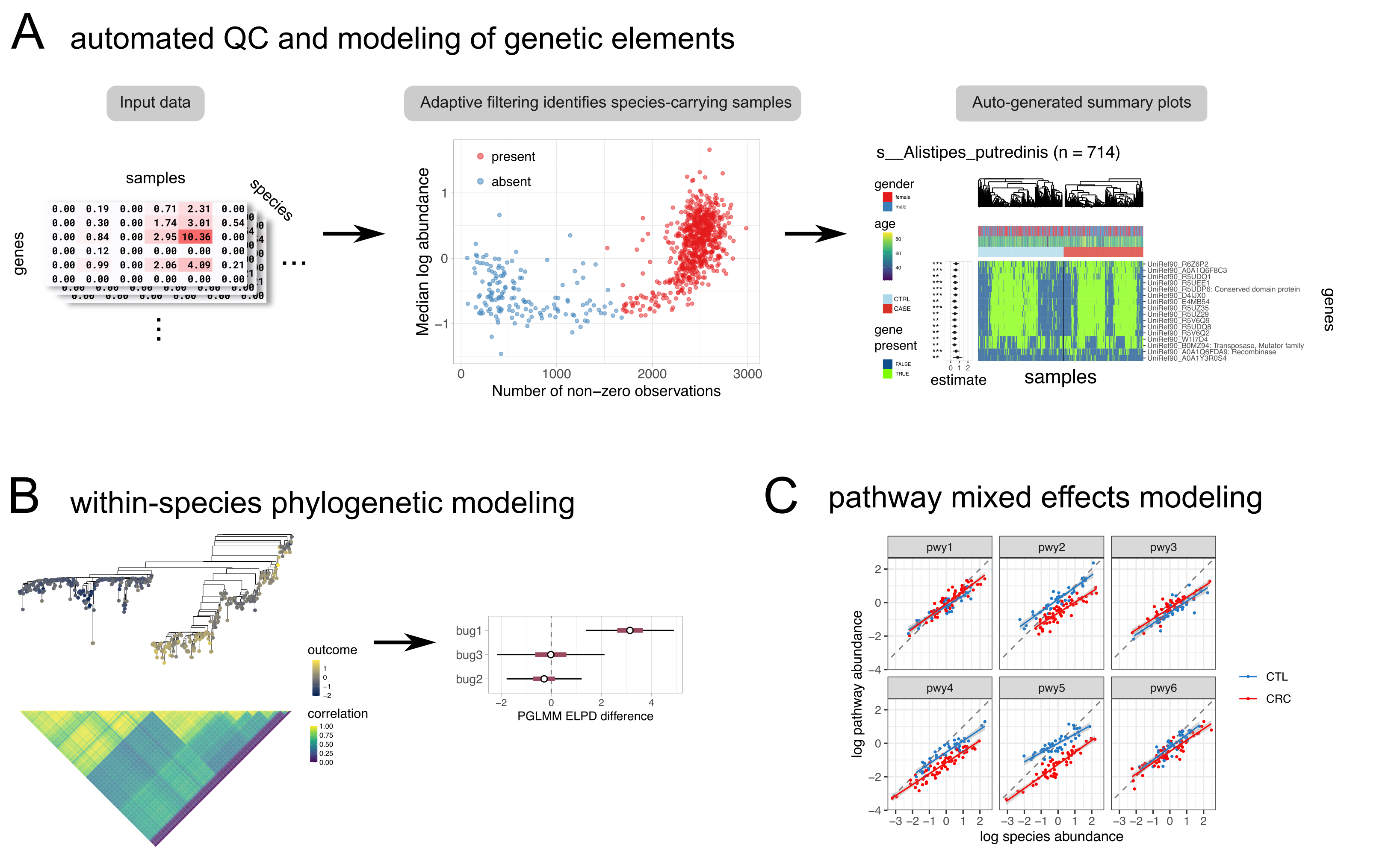
Genetic and genomic variation among microbial strains can dramatically influence their phenotypes and environmental impact, including on human health. However, inferential methods for quantifying these differences have been lacking. Strain-level metagenomic profiling data has several features that make traditional statistical methods challenging to use, including high dimensionality, extreme variation among samples, and complex phylogenetic relatedness. We present Anpan, a set of quantitative methods addressing three key challenges in microbiome strain epidemiology. First, adaptive filtering designed to interrogate microbial strain gene carriage is combined with linear models to identify strain-specific genetic elements associated with host health outcomes and other phenotypes. Second, phylogenetic generalized linear mixed models are used to characterize the association of sub-species lineages with such phenotypes. Finally, random effects models are used to identify pathways more likely to be retained or lost by outcome-associated strains. We validated our methods by simulation, showing that we achieve more accurate effect size estimation and a lower false positive rate compared to alternative methodologies. We then applied our methods to a dataset of 1,262 colorectal cancer patients, identifying functionally adaptive genes and strong phylogenetic effects associated with CRC status, sometimes complementing and sometimes extending known species-level microbiome CRC biomarkers. Anpan’s methods have been implemented as a publicly available R library to support microbial community strain and genetic epidemiology in a variety of contexts, environments, and phenotypes.

User manual || Forum || Tutorial

Citation:

Andrew R. Ghazi^1,2, Kelsey N. Thompson^1,2,4, Amrisha Bhosle^1,2,4, Zhendong Mei³, Yan Yan¹, Fenglei Wang⁵, Kai Wang⁶, Eric A. Franzosa^1,2,4, Curtis Huttenhower^1,2,4,7

Quantifying Metagenomic Strain Associations from Microbiomes with Anpan (In-prep)

¹ Department of Biostatistics, Harvard T.H. Chan School of Public Health, Boston, MA, USA
² Infectious Disease and Microbiome Program, Broad Institute of MIT and Harvard, Cambridge, MA, USA
³ Channing Division of Network Medicine, Department of Medicine, Brigham and Women's Hospital and Harvard Medical School, Boston, MA, USA
⁴ The Harvard Chan Microbiome in Public Health Center, Boston, MA, USA
⁵ Department of Nutrition, Harvard T.H. Chan School of Public Health, Boston, MA, USA
⁶ Department of Epidemiology, Harvard T.H. Chan School of Public Health, Boston, MA, USA
⁷ Department of Immunology and Infectious Diseases, Harvard T.H. Chan School of Public Health, Boston, MA, USA

Overview

Installation

Once you have the dependencies, you can install anpan from github with:

remotes::install_github("biobakery/anpan")

If you would like to read the walkthrough vignette, you will need to set the build_vignettes = TRUE argument in theinstall_github() command, at which point you can view the vignette with vignette("anpan_tutorial", package = 'anpan'). There is also a static (and probably not perfectly up-to-date) version of the tutorial available on the biobakery wiki GitHub page.

Dependencies

anpan depends on R >= 4.1 and the following R packages, most of which are available through CRAN (the exception being cmdstanr):

install.packages(c("ape", 
                   "data.table",
                   "dplyr", 
                   "fastglm",
                   "furrr", 
                   "ggdendro",
                   "ggnewscale",
                   "ggplot2",
                   "loo",
                   "patchwork",
                   "phylogram",
                   "posterior",
                   "progressr",
                   "purrr",
                   "R.utils",
                   "remotes",
                   "stringr",
                   "tibble",
                   "tidyselect")) # add Ncpus = 4 to go faster

install.packages("cmdstanr", repos = c("https://mc-stan.org/r-packages/", getOption("repos")))

If the cmdstanr installation doesn’t work you can find more detailed instructions at this link. Once you’ve installed cmdstanr, you will need to use it to install CmdStan itself:

library(cmdstanr)
check_cmdstan_toolchain()
install_cmdstan(cores = 2)

Example - element testing

You can filter large uniref tables and look for associations with outcomes (while controlling for covariates) withanpan_batch.

library(anpan)

anpan_batch(bug_dir = "/path/to/gene_families/",
            meta_file = "/path/to/metadata.tsv",
            out_dir = "/path/to/output",
            annotation_file = "/path/to/annotation.tsv", #optional, used for plots
            filtering_method = "kmeans",
            model_type = "fastglm",
            covariates = c("age", "gender"),
            outcome = "crc",
            plot_ext = "pdf",
            save_filter_stats = TRUE)

This will run an anpan batch analysis for each functional profile present in bug_dir (there should be one input file per bug). For each bug, anpan:

reads in the metadata (containing the specified outcome and covariates) and the functional profile
applies adaptive filtering to discard samples where the species was likely not present (based on low abundance and few non-zero observations) based on the sample’s functional profile.
fits a model to the filtered data:
- model_type = "fastglm" or model_type = "glm" will fit regressions to each gene in the input file separately (using the specified outcome distribution), then apply FDR correction to the p-values associated with each gene’s presence. The regression for each individual gene follows the form: outcome ~ covariate1 + covariate2 + ... + gene_presence
- model_type = "horseshoe" fits a single regression model with the specified outcome distribution, weak priors on the specified covariates, and a regularized horseshoe prior on the presence/absence of all genes associated with the bug. The regression follows the form: outcome ~ covariate1 + covariate2 + ... + gene1_presence + gene2_presence + gene3_presence + ... including all of the specified covariates and (typically thousands of) genes detected in the bug.
then writes results to the output directory, including tables of regression coefficients, per-bug plots of the top hits, and filter statistics.

Example - phylogenetic generalized linear mixed model

You can run a PGLMM with the anpan_pglmm function. This fits a model where the covariance matrix of outcomes is determined from the phylogenetic tree. Right now the only usable outcome distributions are family = "gaussian" and family = "binomial". If family = "gaussian", the reg_noise parameter can be used to regularize the ratio of the noise parameters with the following prior distribution: $(\sigma_{phylo} / \sigma_{resid}) \sim Gamma(1,2)$

meta_file = "/path/to/metadata.tsv" 
tree_file = "/path/to/file.tre"

anpan_pglmm(meta_file,
tree_file,
trim_pattern = "_bowtie2",
covariates = NULL,
plot_cov_mat = TRUE,
outcome = "age",
verbose = TRUE,
cores = 4)

There is a corresponding anpan_pglmm_batch() function that can be pointed to a directory of .tree files with the tree_dir parameter.